The apcf package provides methods to analyse patterns of objects of finite size and irregular shape using the adapted Pair-Correlation Function (PCF) as proposed by Nuske et al. (2009).
Background
The method suggested by Nuske et al. (2009) requires a certain number of null models for correcting the biased PCF and constructing a pointwise critical envelope. Null models are constructed by randomly moving (shift and rotation) the objects within the study area.
The alpha level of the pointwise critical envelope is according to (Besag and Diggle 1977, Buckland 1984, Stoyan and Stoyan 1994).
For the edge correction (based on Ripley 1981) a buffer with buffer distance is constructed around the object i for each pair of objects i and j. The object j is then weighted by the inverse of the proportion of the buffer perimeter being within the study area.
Being a density function the frequently used Epanechnikov kernel (Silverman 1986, Stoyan and Stoyan 1994) is used for smoothing the PCF. The smoothing is controlled by the bandwith parameter and the step size r. Penttinen et al. (1992) and Stoyan and Stoyan (1994) suggest to set c aka stoyan-parameter of between 0.1 and 0.2 with being the intensity of the pattern.
To separate the computationally intensive part (randomization of the objects and the calculation of the proportion of the buffer inside the study area) from the smoothing of the PCF we use a two step approach:
- calculate distances and buffer fractions for original and randomized patterns
- turn the distances and buffer fractions into a PCF together with a pointwise critical envelope
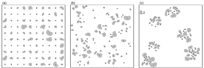
Example Data
To present the workflow we make use of the simulated patterns
presented in Nuske et al. (2009). WKB representations of the data are
part of this package and documented as ?sim_patterns.
Workflow
Pattern to Distances
pat2dists() calculates distances between all object of a
pattern closer than max_dist and determines the fraction of
a buffer with distance dist inside the study area (needed
for edge correction). It randomizes the original pattern to generate
n_sim null models used for correcting the biased PCF and
constructing an envelope. It’s advised against setting
n_sim < 199, better still is 999 or even 9999.
It returns an object of class dists containing a
data.frame with the columns sim, dist, and
prop with an indicator of the model run
(0:n_sim), distances between the objects of the patterns,
and the proportion of a buffer with distance dist inside the study area.
The size of the study area, the total number of objects, and the maximum
distance are passed along as well.
# it's advised against setting n_sim < 199
dists <- pat2dists(area=sim_area, pattern=sim_pat_reg,
                   max_dist=25, n_sim=9, verbose=FALSE)
head(dists)
##   sim     dist     ratio
## 1   0 24.64786 0.9239901
## 2   0 17.15450 1.0000000
## 3   0 20.22583 1.0000000
## 4   0 20.04445 1.0000000
## 5   0 24.13972 0.9517079
## 6   0 19.67695 1.0000000
Distances to PCF
dists2pcf() estimates the adapted pair correlation
function of a pattern of polygons together with a pointwise critical
envelope using kernel methods based on distances between objects.
It returns an object of class fv_pcf containing the
function values of the PCF and the pointwise critical envelope. The
number of null models, the rank of envelope value among the n_sim values
and the bandwith/stoyan parameter are passed along.
pcf <- dists2pcf(dists, r=0.2, r_max=25, stoyan=0.15, n_rank=1)
head(pcf)
## PCF with pointwise critical envelopes
## Obtained from 9 simulations
## Edge correction: "Ripley"
## Alternative: "two.sided"
## Significance level of pointwise Monte Carlo test: 0.2
##
##     r           g       lwr      upr
## 1 0.2 0.000000000 0.7463425 1.269865
## 2 0.4 0.000000000 0.7422944 1.234590
## 3 0.6 0.000000000 0.7676460 1.206157
## 4 0.8 0.000000000 0.7866854 1.186933
## 5 1.0 0.005908318 0.8225105 1.177069
## 6 1.2 0.013306581 0.8623679 1.173386
Plotting the PCF
plot.fv_pcf() is a plot method for the class
fv_pcf. It draws a pair correlation function and a
pointwise critical envelope if available.
plot(pcf)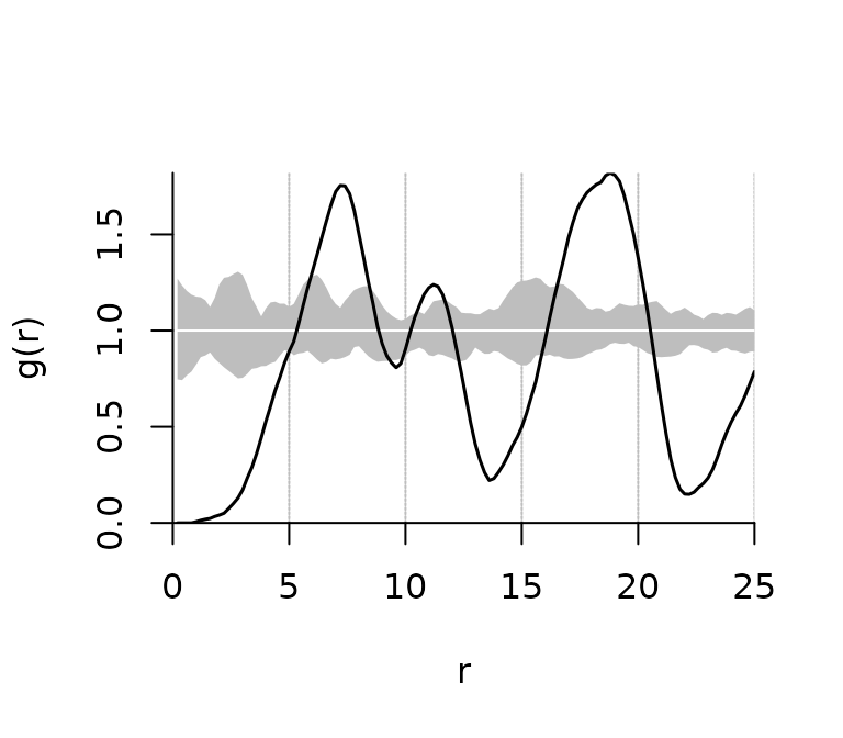
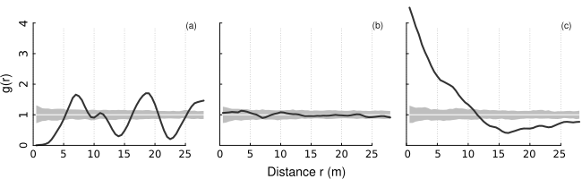
A plot of PCFs of the simulated patterns shown above having (a) regular, (b) random, and (c) clustered objects. Black line: estimated function; white line: theoretical value of the function under the null hypothesis of complete spatial randomness; grey area: 95% confidence envelope under the null hypothesis, computed by Monte Carlo simulation using 199 replicates. Values g(r) < 1 suggest inhibition between points and values g(r) > 1 suggest clustering.
Technical Details
The adapted pair-correlation functions was original implemented in
the Geodatabase PostGIS. PostGIS offers all
necessary geoprocessing methods and is easy to handle knowing databases
and SQL. The need to create many temporary tables and countless
transformations of the geodata stored as WKB in the database into the
“GEOS” format for geometric operations made the process very slow.
In this package the geometric operations (measuring distances between
objects, buffers, intersects, and randomly moving objects) are carried
out by GEOS. The geodata
is read and transformed to GEOS format only once. All
further manipulations are within the GEOS world. Using the
GEOS library from R was made possible by Rcpp.
References
Besag, J. and Diggle, P.J. (1977): Simple Monte Carlo tests for spatial pattern. Journal of the Royal Statistical Society. Series C (Applied Statistics), 26(3): 327–333.
Buckland, S.T. (1984): Monte Carlo Confidence Intervals. Biometrics, 40(3): 811–817.
Nuske, R.S., Sprauer, S. and Saborowski, J. (2009): Adapting the pair-correlation function for analysing the spatial distribution of canopy gaps. Forest Ecology and Management, 259(1): 107–116.
Ripley, B.D. (1981): Spatial Statistics. John Wiley & Sons, New York.
Silverman, B.W. (1986): Density Estimation for Statistics and Data Analysis. Chapman and Hall, London.
Stoyan, D. and Stoyan, H. (1994) Fractals, random shapes and point fields: Methods of geometrical statistics. John Wiley & Sons, Chichester.